Quantizing Transformers
Tilmann E. Bartsch, 21.05.2023
The model size and computational costs of modern neural networks are huge. Both can be significantly reduced by using a method called quantization. This post is a detailed guide on how to quantize neural networks and will build up everything required to perform a simple quantization of Google's transformer-based ViT from scratch.
If you only want to see the code:
- script quantizing an MLP using only numpy,
- GitHub repo numpy-quant implementing a simplistic quantization framework based on numpy.
Intro: From quantizing an MLP to quantizing ViT
Quantizing transformers shows to improve memory usage and inference speed by up to four times - maybe even more then that in the futre. As transformers have become ubiquitous in current advances in the machine learning domain a lot of folks started working on quantizing them. I.e. this, this, this, this and this paper have been published in last few months.
If you are developing transformer architectures and care about inference cost then you should consider how to quantize your networks. Unfortunately, existing tools like Google's tensorflow-lite, Facebook's quantization API or Qualcomm's aimet are complex tools looking like black-boxes from the outside.
Quantization is actually very simple when removing all boilerplate. In part I of this post a ~100 line standalone MLP quantization script (source) using only numpy will be developed which quantizes a simple MLP trained on a circles dataset.
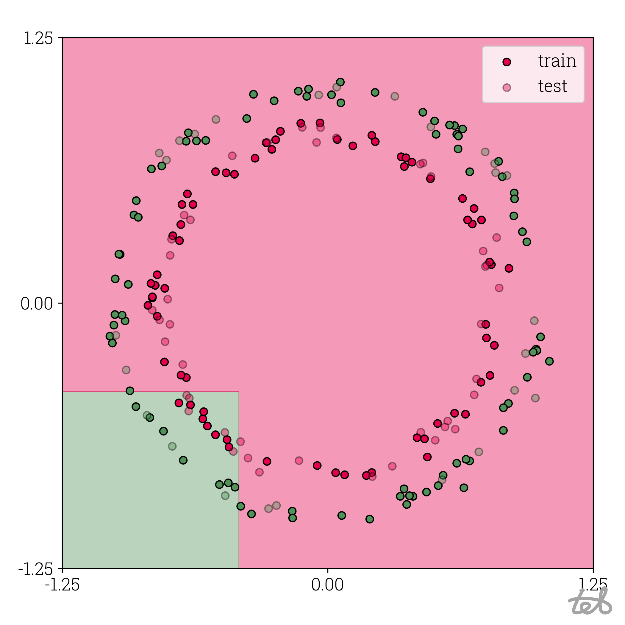
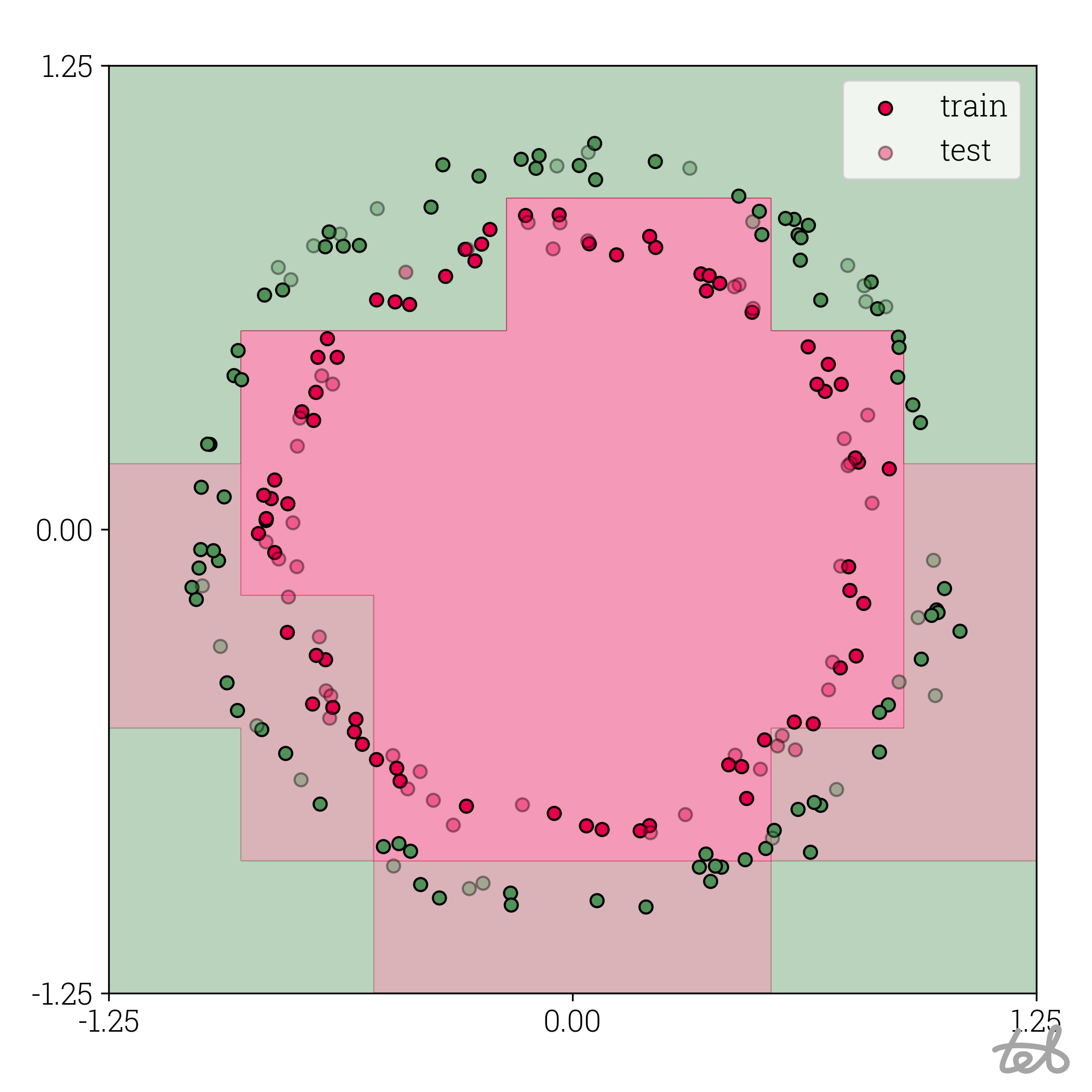
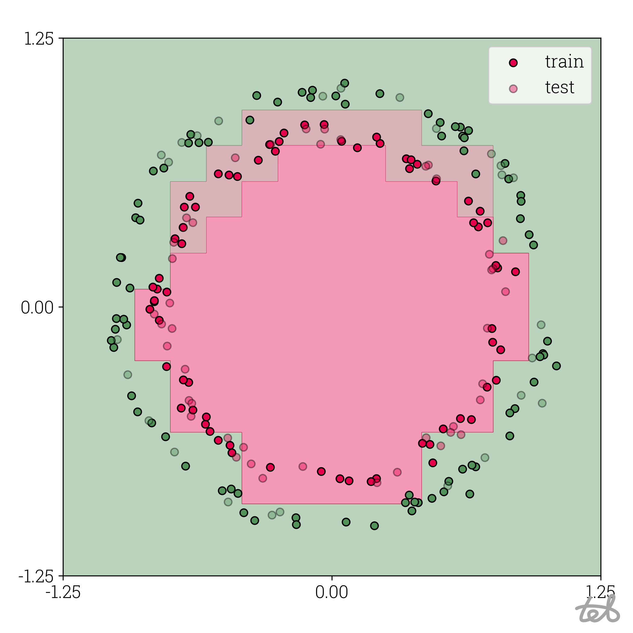
As an appetizer: the effect of quantization for the MLP trained on a circles dataset can be visualized like this:
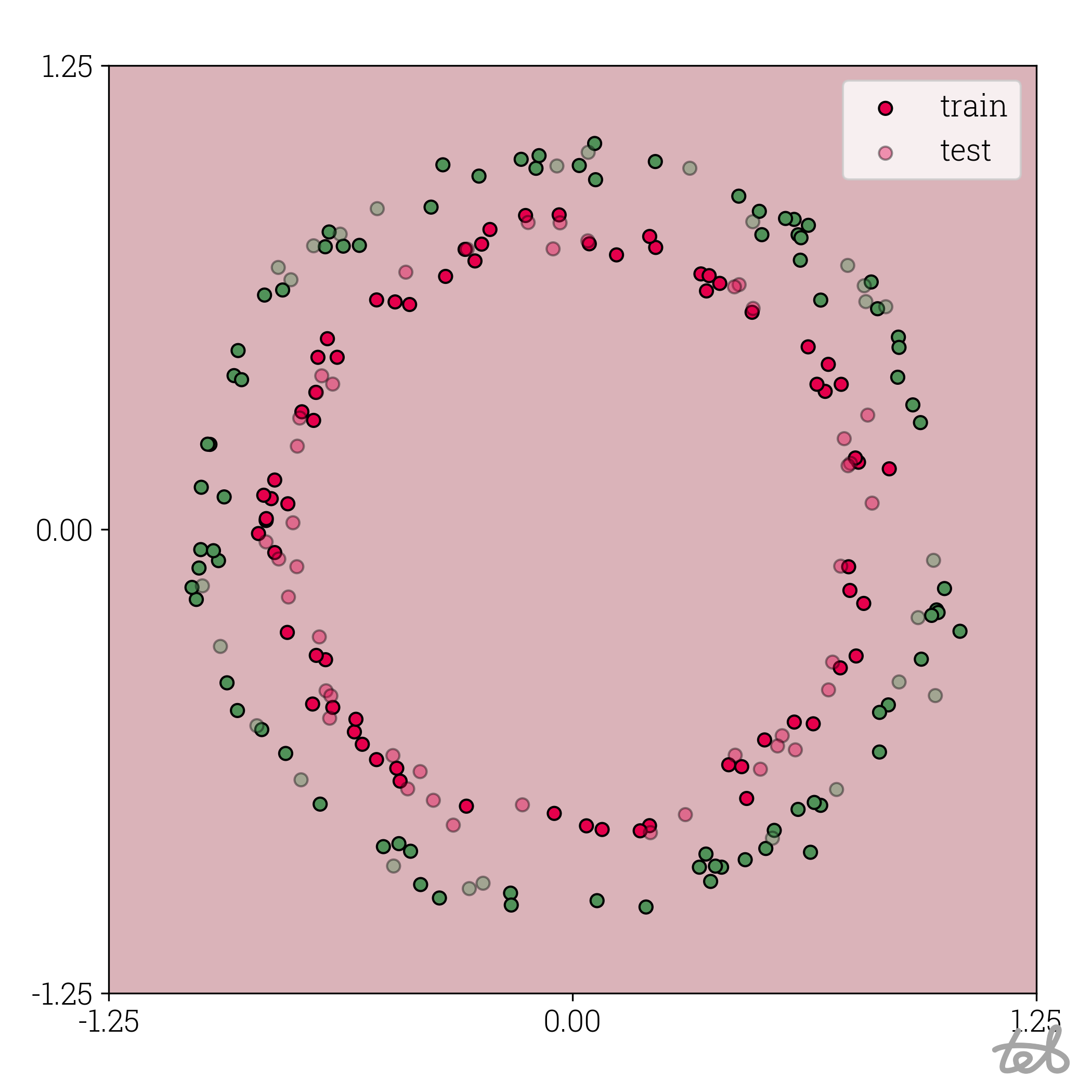 Circle dataset with 1-bit quantized MLP contour plot
 Circle dataset with 2-bit quantized MLP contour plot
 Circle dataset with 3-bit quantized MLP contour plot
 Circle dataset with 4-bit quantized MLP contour plot
 Circle dataset with 5-bit quantized MLP contour plot
 Circle dataset with 6-bit quantized MLP contour plot
 Circle dataset with 8-bit quantized MLP contour plot
 Circle dataset with 10-bit quantized MLP contour plot
 Circle dataset with f32 MLP contour plot
Part II will show how to use this idea to build a simplistic quantization framework able to quantize ViT.
Part I: Quantizing an MLP in 120 lines of code
In this part, we will develop a python script which quantizes a multi-layer-perceptron (MLP) in <120 lines of code using only numpy. For that, we follow three steps:
- quantize an example tensor,
- quantize an example matrix-matrix multiplication,
- quantize a simple MLP.
By covering the quantization of (general) matrix-matrix multiplication, we are able to quantize dense layers as well as matrix-mulitplication-layers enabling to quantize ViT in Part II.
All code snippets in this part are designed to work isolated. They are meant to be executed and played with while reading this post. Don't be discouraged by the increasing size of the snippets. Only a few lines of new code is added in every listing.
A simple start: Quantizing tensors
Quantizing a tensor is a straightforward endeavor. I.e. for int8-quantization it corresponds to rescaling and
round the float32 values of a tensor to integers between -128 to 127 represented by int8-numbers.
More formally, we can consider a tensor x\in\mathbb{R}^{m\times n} and aim to represent x by a tensor q_x\in\lbrace-2^k,\dots,2^k-1\rbrace (k representing the bit width), a zero point z_x\in\lbrace-2^k,\dots,2^k-1\rbrace and a scale s_x\in\mathbb{R} such that:
For given s_x and z_x we can compute (\lfloor.\rceil denotes rounding to the nearest integer)
and test the quantization error by inserting the resulting q_x into \eqref{eqn:tensor_quantization}.
A numpy implementation of this can be done like so:
import numpy as np

arr = np.array([[ 4.4037123 ], [-2.9683902 ], [-4.4077654 ], [ 2.3313837 ], [ 0.05330967]], dtype=np.float32)

def quantize(data: np.ndarray, scale: float, zero_point: int, bit_width: int):
    q_data = zero_point + data / scale

    min_qval, max_qval = -2.0 ** (bit_width - 1), 2.0 ** (bit_width - 1) - 1.0
    # Rescaled numbers which are smaller than the minimum quantized value `min_qval` are clipped to
    # this minimum value. Analogously for rescaled numbers greater than `max_qval`.
    q_data_clipped = np.clip(q_data, min_qval, max_qval)
    q_data_boxed = np.array(np.rint(q_data_clipped), dtype=np.int64)

    return q_data_boxed

def dequantize(arr: np.ndarray, scale: float, zero_point: int | np.ndarray):
    return ((arr - zero_point) * scale).astype(np.float32)

# We choose scaling parameters which rescale the data approximately to an interval of -128 to 127
scale = 0.04
zero_point = 0

arr_quantized = quantize(arr, scale, zero_point, bit_width=8)
arr_round_trip = dequantize(arr_quantized, scale, zero_point)

with np.printoptions(precision=4, suppress=True):
    print("arr:\n", np.array2string(arr))
    print("arr_quantized:\n", np.array2string(arr_quantized))
    print("arr_round_trip:\n", np.array2string(arr_round_trip))
    print("round-trip error:\n", np.abs(arr - arr_round_trip))
The code above yields the following result, in which we observe that the quantization/dequantization round-trip error is ~1%.
| f32 origin | int8 quantized | f32 round-tripped | round-trip error | |||
|---|---|---|---|---|---|---|
| 4.4037 | 110 | 4.4000 | 0.0037 | |||
| -2.9684 | -74 | -2.9600 | 0.0084 | |||
| -4.4078 | -110 | -4.4000 | 0.0078 | |||
| 2.3314 | 58 | 2.3200 | 0.0114 | |||
| 0.0533 | 1 | 0.0400 | 0.0133 |
In the current code the scale and zero_point are chosen arbitrarily. The easiest way to obtain those parameters
is using the tensor's minimum and maximum value. This procedure can be found in the function quant_parameters below,
which implements two quantization modes, namely
- symmetric quantization: Setting
zero_pointto0and calculatingscaleto fit into, - asymmetric quantization: Setting
zero_pointto a value other than0to amend the case the tensor's values are not distributed equally around zero.
import numpy as np

arr = np.array([[ 4.4037123 ], [-2.9683902 ], [-4.4077654 ], [ 2.3313837 ], [ 0.05330967]], dtype=np.float32)

def quantize(data: np.ndarray, scale: float, zero_point: int, bit_width: int):
    q_data = zero_point + data / scale

    min_qval, max_qval = -2.0 ** (bit_width - 1), 2.0 ** (bit_width - 1) - 1.0
    # Rescaled numbers which are smaller than the minimum quantized value `min_qval` are clipped to
    # this minimum value. Analogously for rescaled numbers greater than `max_qval`.
    q_data_clipped = np.clip(q_data, min_qval, max_qval)
    q_data_boxed = np.array(np.rint(q_data_clipped), dtype=np.int64)

    return q_data_boxed

def dequantize(arr: np.ndarray, scale: float, zero_point: int | np.ndarray):
    return ((arr - zero_point) * scale).astype(np.float32)

def quant_parameters(min_val: np.float32, max_val: np.float32, bit_width: int, asymmetric: bool):
    min_qval, max_qval = -2.0 ** (bit_width - 1), 2.0 ** (bit_width - 1) - 1.0

    if asymmetric:
        scale = (max_val - min_val) / (max_qval - min_qval)
        zero_point0 = min_qval - min_val / scale
        zero_point = np.rint(zero_point0).astype(np.int64)
    else:
        scale = (2 * max(max_val, min_val)) / (max_qval - min_qval)
        zero_point = np.array(0, np.int64)

    return scale, zero_point

scale, zero_point = quant_parameters(arr.min(), arr.max(), bit_width=8, asymmetric=True)

arr_quantized = quantize(arr, scale, zero_point, bit_width=8)
arr_round_trip = dequantize(arr_quantized, scale, zero_point)

with np.printoptions(precision=4, suppress=True):
    print(f"scale = {scale}, zero_point = {zero_point}")
    print("arr:\n", np.array2string(arr))
    print("arr_quantized:\n", np.array2string(arr_quantized))
    print("arr_round_trip:\n", np.array2string(arr_round_trip))
    print("round-trip error:\n", np.abs(arr - arr_round_trip))
This code calculates scale == 0.0346, zero_point == 0 as well as a table similar to the one above.
Repeating the procedure for varying bit widths by adjusting the corresponding parameter in the script allows to compare the quantization error for different quantization intensities:
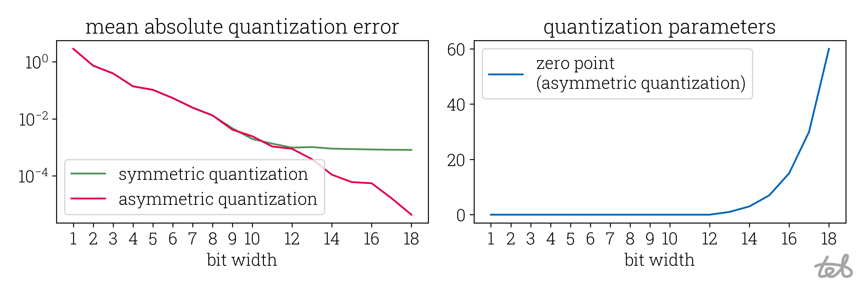 This plot shows the quantization/dequantization round-trip error for the tensor
[4.4, -3.0, -4.4, 2.3, 0.0] as defined in the script above as well as the corresponding zero point
used in asymmetric quantization. The error decreases exponentially with respect
to the used bit width. Note that the mean absolute error of the symmetric quantization
saturates around a bit width of 12 which corresponds to the bit width at which a zero point unequal to
zero is used in asymmetric quantization.
This tells us nothing about the quality of quantization yet because in the end the accuracy drop of a complete network is the only relevant parameter. We'll come back to that later.
Note: The rescaling operation could be formulated in different manners as well, i.e.
scale * (zero_point + data). See gemmlowp's quantization tutorial for details why these alternatives are not used.
Into the rabbit hole: Quantizing a matrix-matrix multiplication
Before implementing quantized matrix-matrix multiplication we formulate the basic idea as has been done in Benoit et al.'s quantization paper.
For floating point tensors, x_1\in\mathbb{R}^{k\times m} and x_2\in\mathbb{R}^{m\times n} and their matrix multiplication w=x_1\cdot x_2 we write similar to above
Now since w=x_1\cdot x_2 we can assume
Which can be rearranged to
Be aware of the sloppy notation used in the terms z_{x_1}q_{x_2} and z_{x_2}q_{x_1} and z_{x_1}z_{x_2}: i.e. z_{x_1} has to be considered as a matrix of shape x_1 with the element z_{x_1} at each position.
Before implementing this, we divide \eqref{eqn:quantized_matmul} into two parts:
-
Calculate q_y, s_y and z_y. This is called quantized matrix-matrix multiplication. Note that
- q_y requires a higher bit-width to represent than q_{x_1} and q_{x_2}. Otherwise, an overflow would occur very easily. The common approach is to represent q_{x_1} and q_{x_2} width 8 bits and q_y with 32 bits.
- the zero point z_y is actually a matrix of the same shape as q_y.
-
Calculate (\lfloor.\rceil denotes rounding to the nearest integer)
\qquad q_w = \left\lfloor z_w + \frac{s_y}{s_w}\cdot(q_y - z_y)\right\rceil
This step is called requantization.
We proceed by baking these formulas into another standalone script.
import numpy as np

x1 = np.array([[-0.68969274,  0.36898366], [ 0.48721004,  0.59565425], [ 0.9734074 , -0.08323386]], dtype=np.float32)
x2 = np.array([[ 4.4037123 , -2.9683902 , -4.4077654 ,  2.3313837 ,  0.05330967], [-1.0420023 ,  3.5323772 , -1.5059234 ,  4.3279686 , -4.243471  ]], dtype=np.float32)

def quantize(data: np.ndarray, scale: float, zero_point: int, bit_width: int):
    q_data = zero_point + data / scale

    min_qval, max_qval = -2.0 ** (bit_width - 1), 2.0 ** (bit_width - 1) - 1.0
    # Rescaled numbers which are smaller than the minimum quantized value `min_qval` are clipped to
    # this minimum value. Analogously for rescaled numbers greater than `max_qval`.
    q_data_clipped = np.clip(q_data, min_qval, max_qval)
    q_data_boxed = np.array(np.rint(q_data_clipped), dtype=np.int64)

    return q_data_boxed

def dequantize(arr: np.ndarray, scale: float, zero_point: int | np.ndarray):
    return ((arr - zero_point) * scale).astype(np.float32)

def quant_parameters(min_val: np.float32, max_val: np.float32, bit_width: int, asymmetric: bool):
    min_qval, max_qval = -2.0 ** (bit_width - 1), 2.0 ** (bit_width - 1) - 1.0

    if asymmetric:
        scale = (max_val - min_val) / (max_qval - min_qval)
        zero_point0 = min_qval - min_val / scale
        zero_point = np.rint(zero_point0).astype(np.int64)
    else:
        scale = (2 * max(max_val, min_val)) / (max_qval - min_qval)
        zero_point = np.array(0, np.int64)

    return scale, zero_point

def q_matmul(arr_a: np.ndarray, scale_a: float, zero_point_a: int,
           arr_b: np.ndarray, scale_b: float, zero_point_b: int):
    q_matmul_result = np.matmul(arr_a.astype(np.int64), arr_b)
    scale = scale_a * scale_b
    zero_points = (arr_a.sum(axis=-1, keepdims=True) * zero_point_b
                  + arr_b.sum(axis=-2, keepdims=True) * zero_point_a
                  - zero_point_a * zero_point_b * arr_a.shape[-1])
    return q_matmul_result, scale, zero_points

def requantize(arr: np.ndarray, arr_scale: float, arr_zero_points: np.ndarray,
               res_scale: float, res_zero_point: int, bit_width: int):
    min_qval, max_qval = -2.0 ** (bit_width - 1), 2.0 ** (bit_width - 1) - 1.0
    dequant = dequantize(arr, arr_scale, arr_zero_points)
    qdata = np.clip(np.rint(res_zero_point + 1 / res_scale * dequant), min_qval, max_qval).astype(np.int64)
    return qdata

# Float matrix multiplication
w_f32 = np.matmul(x1, x2)

# Quantize input arrays
x1_scale, x1_zero_point = quant_parameters(x1.min(), x1.max(), bit_width=8, asymmetric=True)
x2_scale, x2_zero_point = quant_parameters(x2.min(), x2.max(), bit_width=8, asymmetric=True)
x1_quant = quantize(x1, x1_scale, x1_zero_point, bit_width=8)
x2_quant = quantize(x2, x2_scale, x2_zero_point, bit_width=8)

# Perform matrix multiplication. Result is quantized with a higher bit width, i.e. for `bit_width == 8`
# the elements of result `q_mm` have a bit_width of 32.
y, y_scale, y_zero_points = q_matmul(x1_quant, x1_scale, x1_zero_point, x2_quant, x2_scale, x2_zero_point)

# Requantize to original bit_width, i.e. 8. For that use quantization parameters obtained from `f32_matmul`.
w_scale, w_zero_point = quant_parameters(w_f32.min(), w_f32.max(), bit_width=8, asymmetric=True)
w_quant = requantize(y, y_scale, y_zero_points,
                     w_scale, w_zero_point, bit_width=8)

# Dequantize result
w_round_trip = dequantize(w_quant, w_scale, w_zero_point)

with np.printoptions(precision=4, suppress=True):
    print("w_f32:\n", np.array2string(w_f32))
    print("w_round_trip:\n", np.array2string(w_round_trip))
    print("round-trip error:\n", np.abs(w_f32 - w_round_trip))
which prints the following three (3x5)-arrays:
| f32 matmul | quantized matmul | error | ||||||||||||||
|---|---|---|---|---|---|---|---|---|---|---|---|---|---|---|---|---|
| -3.4217 | 3.3507 | 2.4843 | -0.0110 | -1.6025 | -3.4154 | 3.3484 | 2.4779 | 0.0000 | -1.6407 | 0.0063 | 0.0022 | 0.0065 | 0.0110 | 0.0382 | ||
| 1.5249 | 0.6578 | -3.0445 | 3.7138 | -2.5017 | 1.5403 | 0.6362 | -3.0806 | 3.6833 | -2.4779 | 0.0154 | 0.0216 | 0.0361 | 0.0306 | 0.0238 | ||
| 4.3733 | -3.1835 | -4.1652 | 1.9092 | 0.4051 | 4.3530 | -3.1810 | -4.1521 | 1.8751 | 0.4353 | 0.0204 | 0.0024 | 0.0131 | 0.0340 | 0.0302 |
Like above, we can compare the approximation quality:
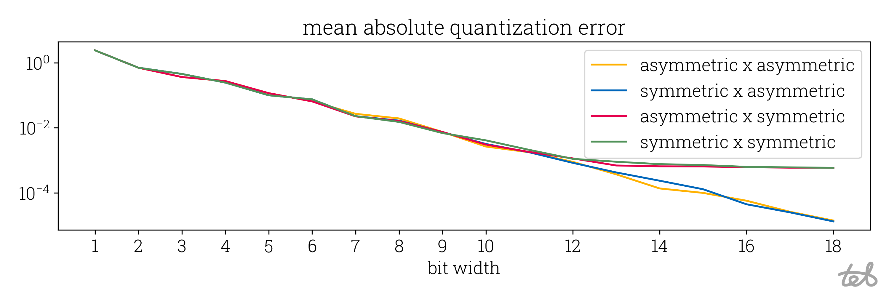 Mean absolute quantization error of the quantized matrix-matrix multiplication as implemented
in the code above. Each combination of symmetric/asymmetric quantization of the input matrix
is evaluated. The error reduces exponentially with the bit width and saturates around a bit width
of 13 if the second matrix is quantized symmetrically.
Mean absolute quantization error of the quantized matrix-matrix multiplication as implemented
in the code above. Each combination of symmetric/asymmetric quantization of the input matrix
is evaluated. The error reduces exponentially with the bit width and saturates around a bit width
of 13 if the second matrix is quantized symmetrically.
Stringing it together: Obtaining an MLP's quantization accuracy drop
We finalize the first part by quantizing a very simple MLP with a single hidden layer, which is trained on a non-linear circles-dataset. See this file for the exact model definition and training procedure.
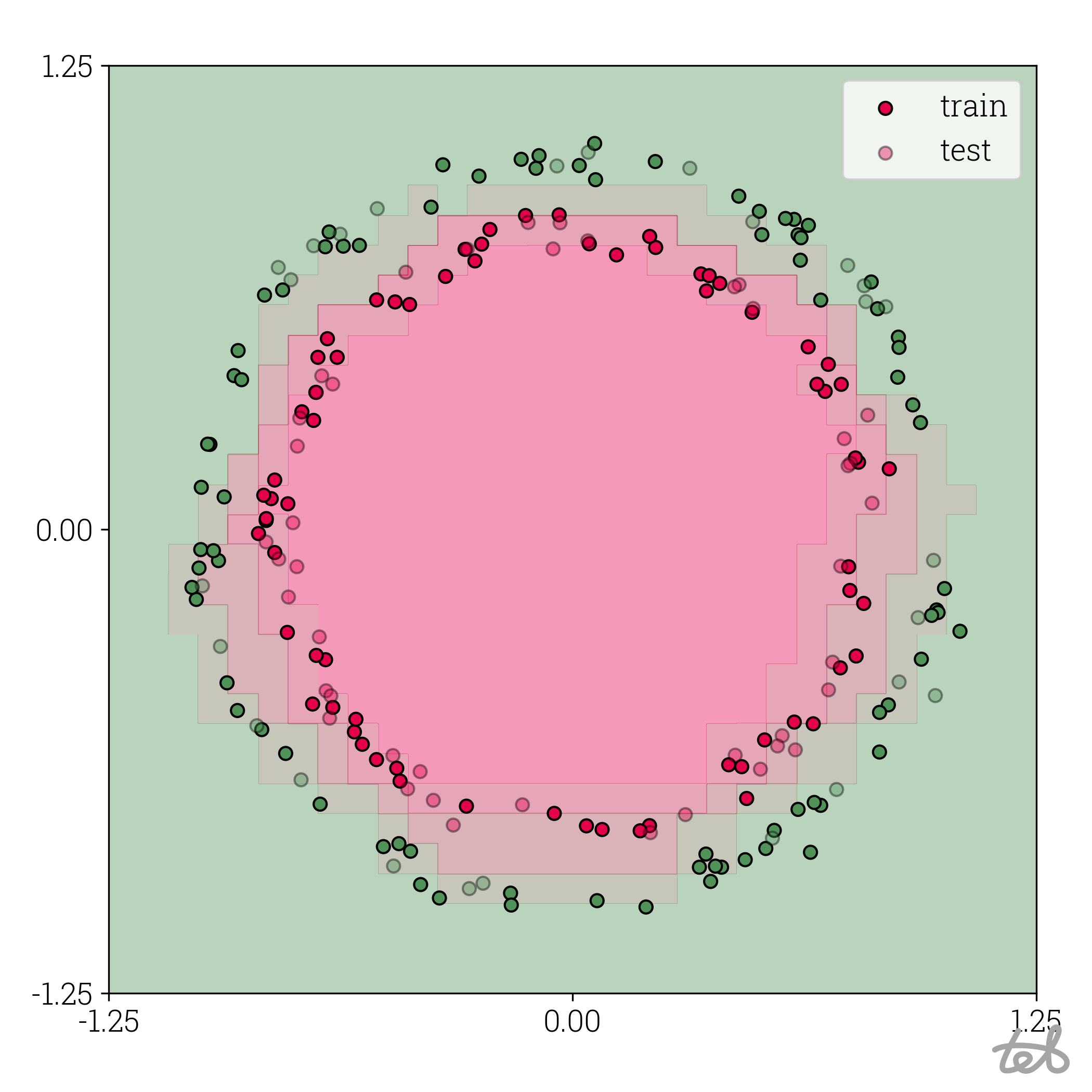
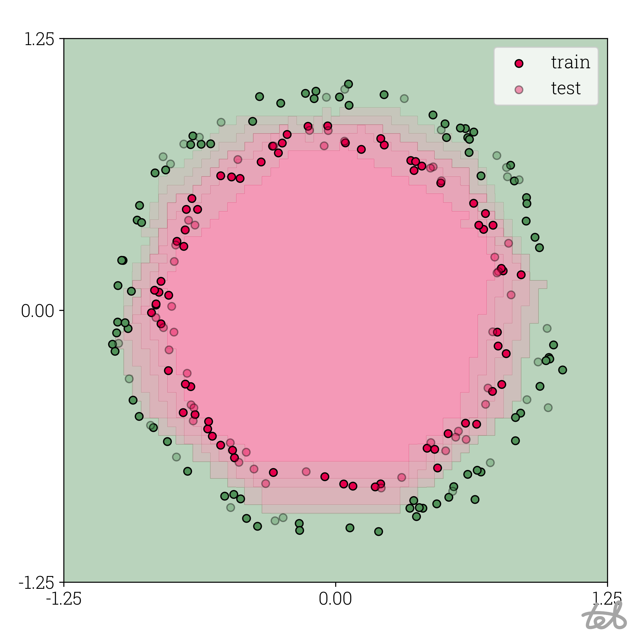
In the following image, we can see the utilized dataset containing of x- and y-locations as features and one of two classes (green or red) as label/target. Furthermore, the trained model is evaluated on a close-meshed grid to obtain a contour plot:
Visualization of circle dataset with two classes. The features are the x and y
position of every dot and the color corresponds to one of the two possible targets/labels. In the background
the contour plot of an MLP trained on this dataset is shown.
Before we are able to quantize this MLP, we have to adjust our current formula derived from \eqref{eqn:matmul_quantization_start_point} to support bias. For that we denote x_1\in\mathbb{R}^{k\times m}, x_2\in\mathbb{R}^{m\times n} and b\in\mathbb{R}^{k\times n} and general matrix multiplication w=x_1\cdot x_2 + b. Using the notation from above, we obtain
Which means that we can support a bias in the quantized matrix multiplication by
-
Quantizing b to q_b with scale s_{x_1}s_{x_2} and zero point 0 such that
\qquad b \approx s_{x_1}s_{x_2}\cdot q_b
-
Performing quantized general matrix-matrix multiplication by calculating q_y=q_{x_1}q_{x_2}+q_b as well as s_y=s_{x_1}s_{x_2} and z_y=-z_{x_1}q_{x_2}-z_{x_2}q_{x_1}+z_{x_1}z_{x_2}.
-
Requantize the result the same way as before by calculating
\qquad q_w = \left\lfloor z_w + \frac{s_y}{s_w}\cdot(q_y - z_y)\right\rceil
Writing everything down, we get an MLP quantization script containing less than 120 lines of code:
import numpy as np

# Quantization routines

def quantize(data: np.ndarray, scale: float, zero_point: int, bit_width: int):
    q_data = zero_point + data / scale

    min_qval, max_qval = -2.0 ** (bit_width - 1), 2.0 ** (bit_width - 1) - 1.0
    # Rescaled numbers which are smaller than the minimum quantized value `min_qval` are clipped to
    # this minimum value. Analogously for rescaled numbers greater than `max_qval`.
    q_data_clipped = np.clip(q_data, min_qval, max_qval)
    q_data_boxed = np.array(np.rint(q_data_clipped), dtype=np.int64)

    return q_data_boxed

def dequantize(arr: np.ndarray, scale: float, zero_point: int | np.ndarray):
    return ((arr - zero_point) * scale).astype(np.float32)

def quant_parameters(min_val: np.float32, max_val: np.float32, bit_width: int, asymmetric: bool):
    min_qval, max_qval = -2.0 ** (bit_width - 1), 2.0 ** (bit_width - 1) - 1.0

    if asymmetric:
        scale = (max_val - min_val) / (max_qval - min_qval)
        zero_point0 = min_qval - min_val / scale
        zero_point = np.rint(zero_point0).astype(np.int64)
    else:
        scale = (2 * max(max_val, min_val)) / (max_qval - min_qval)
        zero_point = np.array(0, np.int64)

    return scale, zero_point

def q_matmul(arr_a: np.ndarray, scale_a: float, zero_point_a: int,
           arr_b: np.ndarray, scale_b: float, zero_point_b: int):
    q_matmul_result = np.matmul(arr_a.astype(np.int64), arr_b)
    scale = scale_a * scale_b
    zero_points = (arr_a.sum(axis=-1, keepdims=True) * zero_point_b
                  + arr_b.sum(axis=-2, keepdims=True) * zero_point_a
                  - zero_point_a * zero_point_b * arr_a.shape[-1])
    return q_matmul_result, scale, zero_points

def requantize(arr: np.ndarray, arr_scale: float, arr_zero_points: np.ndarray,
               res_scale: float, res_zero_point: int, bit_width: int):
    min_qval, max_qval = -2.0 ** (bit_width - 1), 2.0 ** (bit_width - 1) - 1.0
    dequant = dequantize(arr, arr_scale, arr_zero_points)
    qdata = np.clip(np.rint(res_zero_point + 1 / res_scale * dequant), min_qval, max_qval).astype(np.int64)
    return qdata

# Trained MLP for circles dataset

# # Every row of `inp` contains the x and y position of a point
inp = np.array([[0., 0.], [1., 1.]], dtype=np.float32)

fc1_weight = np.array([[ 4.4037123 , -2.9683902 , -4.4077654 ,  2.3313837 ,  0.05330967], [-1.0420023 ,  3.5323772 , -1.5059234 ,  4.3279686 , -4.243471  ]], dtype=np.float32)
fc1_bias = np.array([-2.0229015, -2.446563 , -2.7381809, -2.715235 , -1.9951458], dtype=np.float32)
fc2_weight = np.array([[ 2.7341564, -2.7900338], [ 3.049221 , -3.114146 ], [ 2.761332 , -2.8246257], [ 3.0681298, -3.1184993], [ 2.8039508, -2.8363247]], dtype=np.float32)
fc2_bias = np.array([-4.372014,  4.457383], dtype=np.float32)

fc1_out = np.matmul(inp, fc1_weight) + fc1_bias  # dense layer #1
fc1_act = fc1_out.copy()
fc1_act[fc1_out < 0] = 0.0  # first layer activation  # activation #1 (relu)
fc2_out = np.matmul(fc1_act, fc2_weight) + fc2_bias  # dense layer #2
fc2_act = 1.0 / (1.0 + np.exp(-fc2_out))  # activation #2 (sigmoid)

# Quantize MLP

# # Input
inp_scale, inp_zero_point = quant_parameters(inp.min(), inp.max(), bit_width=8, asymmetric=True)
inp_q = quantize(inp, inp_scale, inp_zero_point, bit_width=8)

# # FC layer 1
fc1_weight_scale, fc1_weight_zero_point = quant_parameters(fc1_weight.min(), fc1_weight.max(), bit_width=8, asymmetric=False)
fc1_weight_q = quantize(fc1_weight, fc1_weight_scale, fc1_weight_zero_point, bit_width=8)
fc1_out_scale, fc1_out_zero_point = quant_parameters(fc1_out.min(), fc1_out.max(), bit_width=8, asymmetric=True)
fc1_bias_q = quantize(fc1_bias, inp_scale * fc1_weight_scale, 0, bit_width=32)

# # FC layer 2
fc2_weight_scale, fc2_weight_zero_point = quant_parameters(fc2_weight.min(), fc2_weight.max(), bit_width=8, asymmetric=False)
fc2_weight_q = quantize(fc2_weight, fc2_weight_scale, fc2_weight_zero_point, bit_width=8)
fc2_out_scale, fc2_out_zero_point = quant_parameters(fc2_out.min(), fc2_out.max(), bit_width=8, asymmetric=True)
fc2_bias_q = quantize(fc2_bias, fc1_out_scale * fc2_weight_scale, 0, bit_width=32)

# Run inference using quantized MLP

# # FC layer 1
fc1_y, fc1_y_scale, fc1_y_zero_points = q_matmul(inp_q, inp_scale, inp_zero_point,
                                                 fc1_weight_q, fc1_weight_scale, fc1_weight_zero_point)
fc1_out_q = requantize(fc1_y + fc1_bias_q, fc1_y_scale, fc1_y_zero_points,
                       fc1_out_scale, fc1_out_zero_point, bit_width=8)

# # ReLU activation
fc1_act_q = fc1_out_q.copy()
fc1_act_q[fc1_out_q < fc1_out_zero_point] = fc1_out_zero_point

# # FC layer 2
fc2_y, fc2_y_scale, fc2_y_zero_points = q_matmul(fc1_act_q, fc1_out_scale, fc1_out_zero_point,
                                                 fc2_weight_q, fc2_weight_scale, fc2_weight_zero_point)
fc2_out_q = requantize(fc2_y + fc2_bias_q, fc2_y_scale, fc2_y_zero_points,
                       fc2_out_scale, fc2_out_zero_point, bit_width=8)

# Dequantize output of 2. FC layer
fc2_out_deq = dequantize(fc2_out_q, fc2_out_scale, fc2_out_zero_point)

# # Sigmoid activation on dequantized output of 2. FC layer
fc2_act_deq = 1.0 / (1.0 + np.exp(-fc2_out_deq))

with np.printoptions(precision=4, suppress=True):
    print("fc2_act:\n", np.array2string(fc2_act))
    print("fc2_act_deq:\n", np.array2string(fc2_act_deq))
    print("quantized inference error:\n", np.abs(fc2_act_deq - fc2_act))
( complete script )
Using this code on the test set mentioned above for different bit widths, we can compare the final effectiveness of the implemented quantization:
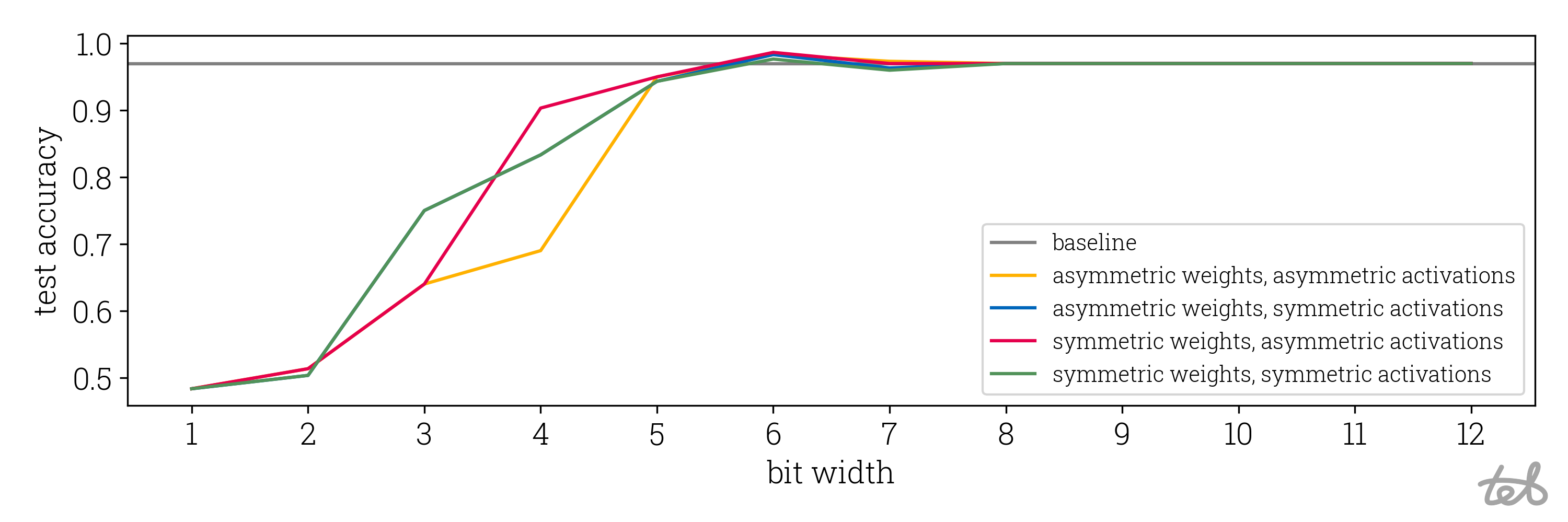 Accuracy of the quantized MLP as performed in the code above on the test split of the circles
dataset. It is clear that using 8-bit quantization results in no relevant accuracy loss. We also see that accuracy
drop saturates at a bit width of about 5.
Accuracy of the quantized MLP as performed in the code above on the test split of the circles
dataset. It is clear that using 8-bit quantization results in no relevant accuracy loss. We also see that accuracy
drop saturates at a bit width of about 5.
Also compare the contour plots of the quantized models to the original float32 model as shown in the introduction
of this post.
Part II: Expanding quantized matrix multiplication to ViT quantization
Having the five quantization functions quantize, dequantize, quant_parameters, q_matmul and requantize
up our sleeves it is possible to build a small framework which is able to quantize ViT and run it
without using any other packages. To achieve this we
- build a graph structure which models the computational graph of ViT imported from ViT
- implement a routine successively computing all tensors in such graphs for a given input tensor
- implement a method producing a modified computational graph representing the quantized network
The code snippets of this part are adapted from the repository numpy-quant which implements all necessary steps.
Getting ready: the graph structure
In order to built the computational graph, we basically create one class for Tensor's and one for Value's such that
the Tensor's are connected to Value's and vice versa.
To see how this works, consider this small part of the whole computational graph of ViT (self-attention):

In order to differentiate between float32 and quantized Tensor's we start by creating one class for each:
class FTensor:
    def __init__(self, data: np.ndarray):
        self._data = data

class QTensor:
    def __init__(self, data: np.ndarray[Any, np.int64], bit_width: int, scale: np.float32,
                 zero_point: np.ndarray[Any, np.int64]):
        self.bit_width = bit_width
        self.scale = scale
        self.zero_point = zero_point
        self._data = data.astype(np.int64)

Tensor = Union[FTensor, QTensor]
(numpy-quant sources here and here )
We now proceed by wrapping the tensors into Value's which are connected to Node's. It's convenient to
distinguish further between constant and variable tensors. The Constant Tensors correspond to trained weights of
a NN while the Variable Tensors represent the Tensor's being calculated during inference.
class Constant:
    def __init__(self, name: str, outputs: List['Node'], data: Tensor = None):
        self.name = name
        self.outputs = outputs  # The nodes which use this Constant's data as input
        self.data = data

class Variable:
    def __init__(self, name: str, inputs: List['Node'], outputs: List['Node'], data: Tensor = None):
        self.name = name
        self.inputs = inputs    # The nodes which produce this Variable's data
        self.outputs = outputs  # The nodes which use this Variable's data as input
        self.data = data

Value = Union[Constant, Variable]
(numpy-quant source here )
The Nodes correspond to all kinds of operations, i.e. Matrix-Matrix-Multiplication, ReLU or Reshape. In order to easily import ONNX we follow the ONNX operator scheme:
class Node:
    def __init__(self, name: str, op: str, attrs: dict[str, Any], inputs: List[Value], outputs: List[Value]):
        self.name = name
        self.op = op            # The type of operation to perform, i.e. matrix multiplication
        self.attrs = attrs      # Attributes configuring the behavior of the operation
        self.inputs = inputs    # The values required to calculate the outputs of the node
        self.outputs = outputs  # The values being calculated by the node
(numpy-quant source here )
Lastly, we represent a complete computational graph by a list of Nodes's and Value's as well as the Variable's
constituting the input and output of the graph:
class Model:
    def __init__(self, nodes: list[Node], values: list[Value], inputs: List[Variable], outputs: List[Variable]):
        self.nodes = nodes
        self.values = values
        self.inputs = inputs
        self.outputs = outputs
(numpy-quant source here )
We are now ready to import an ONNX model representing ONNX into this structure. Since our graph description is very similar to the one ONNX is using, the implementation is straightforward:
- Make the onnx model accessible in python via
onnx.load - Iterate over constants of the onnx model (called initializers in ONNX) and create corresponding
Constant's. - Iterate over the nodes of the onnx models, create corresponding
Node's as well asVariable's for the onnx-node's inputs and outputs.
Details can be found in numpy-quant implementation.
Assuming we have the onnx model available at vit.onnx we can now run:
import onnx
from numpy_quant.model import Model

# Import ONNX model to numpy-quant
onnx_model = onnx.load("vit.onnx")
model = Model.from_onnx(onnx_model)

# Print node, values, inputs and outputs of the model
print(model)
( complete script with onnx model creation )
Bringing the graph to life: Running Inference
Now that we have the ViT graph available, we can set a value for the input tensor and then iterate through
the nodes to create the node's output tensors. Note that due to the import of ViT from ONNX the list model.nodes is
sorted such that a Node's inputs are calculated when it is reached in the list.
model = Model.from_onnx("vit.onnx")
model.inputs[0].data = FTensor(np.random.normal((1, 3, 224, 224)))

# Iterate through nodes updating all variables in the model.
for node in model.nodes:
    inputs = [i.data for i in node.inputs]

    outputs = onnx_operator_implementation(node.op, inputs, node.attrs)

    for o, tensor in zip(node.outputs, outputs):
        o.data = tensor
( complete script )
The somewhat tedious task is to implement all necessary operations in the function
onnx_operator_implementation as has been done
here.
Grand Finale: Running a numpy-quantized ViT
In order to transform the ViT graph to a corresponding quantized execution graph, we create a class to represent the quantized model:
class QuantizationParams:
    def __init__(self, scale: np.float32, zero_point: Union[np.int64, None]):
        self.scale = scale
        self.zero_point = zero_point

class QModel(Model):
    def __init__(self, nodes: list[Node], values: list[Value], inputs: List[Variable], outputs: List[Variable],
                 bit_width: int, quant_params: dict[str, QuantizationParams]):
        """
        quant_params: value name -> quantization parameter
            Store the quantization parameters as obtained by numpy_quant.numpy_quantization.quant_parameters
            for every value in the model.
        """
        super(QModel, self).__init__(nodes, values, inputs, outputs)
        self.bit_width = bit_width
        self.quant_params = quant_params
(numpy-quant source here and here and)
In particular, the quantized model keeps a dictionary storing all quantization parameters. In order to obtain
those parameters for the Variable's a reference input data set must be provided to the quantization routine.
These parameters allow to always convert tensors to their quantized version.
In order to quantize all matrix-matrix-multiplications ("matmul") of ViT we can actually use the same computational graph for the quantized model, only changing the following aspects:
-
during model quantization: (code)
- quantize the data of all
Constants which are used as inputs of matrix-matrix multiplication nodes of the original graph,
- quantize the data of all
-
during quantized inference: (code)
- quantize or requantize all inputs of a matmul node before the node's outputs are calculated
- use quantized matrix multiplication instead of the normal one at every matmul-node
- dequantize all inputs of non-matmul-nodes before the node's outputs are calculated
Having all of this set up we can harvest our fruits and see evaluate the performance drop of the ViT for Image Classification:
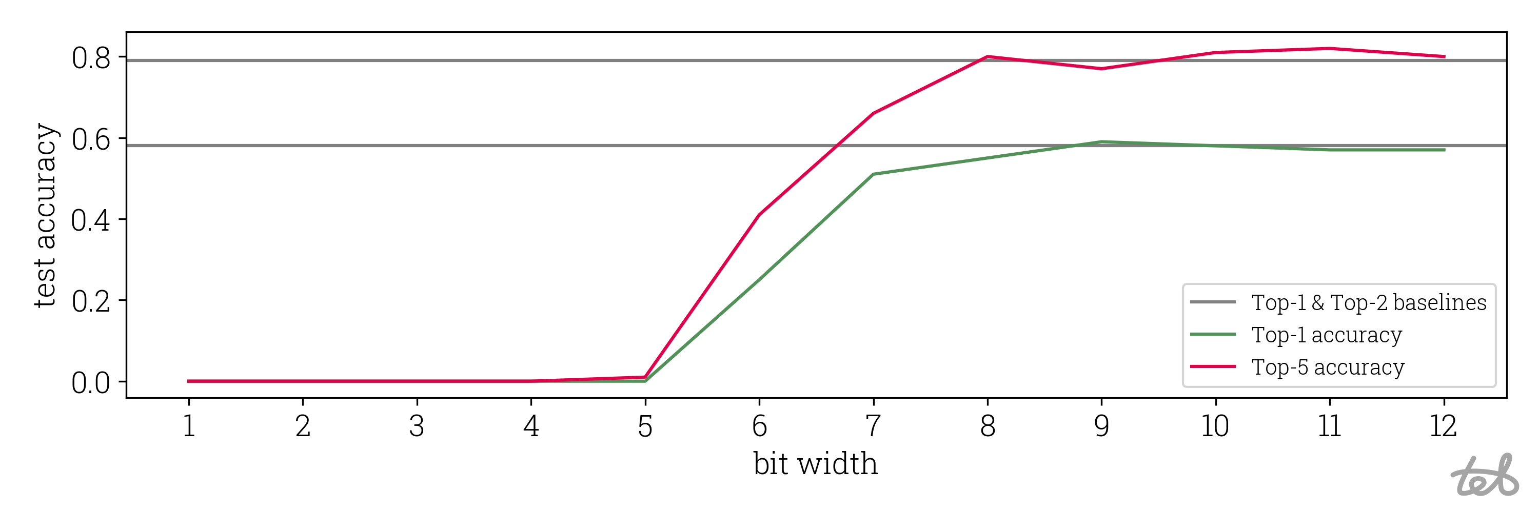 Accuracy drop of presented ViT quantization. The ViT has been adopted from
google/vit-base-patch16-224. Weights are quantized
symmetrically and activations asymmetrically. The accuracy has been calculated using 100 validation images taken from
Maysee/tiny-imagenet.
Accuracy drop of presented ViT quantization. The ViT has been adopted from
google/vit-base-patch16-224. Weights are quantized
symmetrically and activations asymmetrically. The accuracy has been calculated using 100 validation images taken from
Maysee/tiny-imagenet.
Conclusions and where to go next
We have seen that quantizing a neural network as complicated as ViT in python & numpy comes back to
- writing quantization routines in numpy using <75 lines of code
- implementing a computational graph structure modeling ViT
Using that, we found that the simple quantization method developed is able to quantize ViT reasonable well for a bit width of 8 but shows a severe accuracy loss starting at a bit width of 7.
To improve the quality of the acquired quantization, we could i.e. follow one of those methods:
- addressing the fact that the outputs of ViT's GELU and Softmax have a strongly non-gaussian distribution and therefore, are not quantized well (see PTQ4ViT),
- reducing the effect of outliers in the tensors which make quantization ineffective (see this paper),
- quantize besides all operators used by ViT, not only matrix-multiplication, i.e. softmax and layer normalization (see I-ViT and FQ-ViT) or
- in very large transformers (>5 billion parameters) a small number of feature dimensions contain a lot of outliers which prevent simple quantization methods to work. See LLM.int8() and SmoothQuant.

